Guide to Essential Biostatistics XV: Inferential Statistics – Two Sample Means Comparison: the t-Test (Part II)
In the previous articles in this series, we explored the Scientific Method, Proposing Hypotheses and Type-I and Type-II errors, Designing and implementing experiments (Significance, Power, Effect, Variance, Replication, Experimental Degrees of Freedom and Randomization), as well as Critically evaluating experimental data (Q-test; SD, SE, and 95%CI).
In the following articles, we will determine how to accept or reject the hypothesis (f- and t-tests, Chi-square, ANOVA and post-ANOVA testing).
Test statistic – the t-value
The test statistic for all t-tests (one sample, paired two-sample or independent two-sample t-tests) is the t-value or t-ratio, which is the difference between the sample means (numerator) divided by the standard error of the difference (denominator). Expressed in other terms – the numerator is the effect size (signal) and the denominator is the variability (noise) while the t-value may be considered to represent the signal:noise ratio.
The t-values are calculated differently for each test.
- For a one-sample t-test, the expected or theoretical mean is subtracted from the mean of the sample, and this is divided by the standard error of the sample. The degrees of freedom (df) used in this test are n−1. For a sample of 10 seedlings, the degrees of freedom are thus [10-1=9].
- For paired two-sample t-tests, the difference between the sample means is divided by the standard error of the mean differences. As the difference between the sample means is the same as a single sample (the mean differences), the degrees of freedom (df) used in this test are n-1. For two paired samples of 10 seedlings, the degrees of freedom are thus [10-1=9].
- For two-sample t-tests, the difference between the sample means is divided by the pooled (averaged) standard error for the two samples (which in turn explains the need for an assumption of equal variances for the two samples). The degrees of freedom (df) used in this test are [n (sample 1) + n (sample 2) − 2]. For two samples of 10 seedlings, the degrees of freedom are thus [10+10-2=8].
As statistical software packages (and most spreadsheets) provide convenient t-test functions, we will not delve deeper into the calculation of t, but rather focus on interpreting the results.
Example: Comparing treated and untreated seedlings.
In our sample data (see previous article) of the height of ten untreated seedlings compared to the height of ten herbicide-treated seedlings, the f-test was used to determine whether the variances of the two samples were equal or not.
As the f-ratio was smaller than the critical f-value, we could conclude that the variances of the two samples were equal and that we may compare the means using the two-sample t-test for equal variances and calculate or compute the t-value (Figure 1). Had the variances not been equal, we would choose the two-sample t-test for unequal variances.
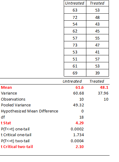
Figure 1: Result of two-sample t-test for equal variances (with p-values) to compare means for two experimental data samples (calculated in Excel).
To interpret the results, the calculated t-value can be compared to two-tail critical t table values (Figure 2) for n-2 degrees of freedom (the total sample size of 10+10-2=18df) to determine whether the sample means are equal (or significantly different):
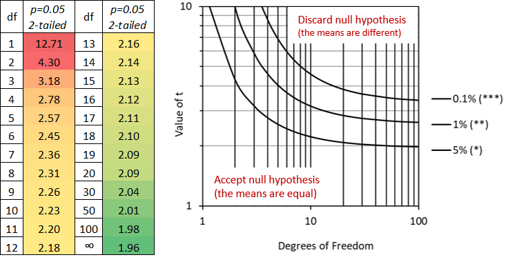
Figure 2: Critical t-values for p= 0.05; two-tailed (left); values of t (two-tailed) for varying levels of significance (right).
As p=0.05 corresponds to a 5% (or less) chance of discarding the null hypothesis (the means are equal), t-values less than the critical table value mean the null hypothesis may not be discarded i.e. the samples have equal means.
In our example, the t-value (4.29) is greater than the critical t-value (t=2.10 for 18df), and we may thus conclude that the means of the two samples are significantly different. Similarly, for our sample data a computed p-value of <0.05 (Figure 1) confirms that the means of the two samples are significantly different.
While t-tests allow us to determine if two samples have the same mean, biological experiments usually comprise more than two samples. Accordingly, Analysis of Variance (ANOVA) tests are used to evaluate multiple (three or more) data samples, and this is the subject of the next articles in this series.
_________________________________
Thanks for reading – please feel free to read and share my other articles in this series!
The first two books in the LABCOAT GUIDE TO CROP PROTECTION series are now published and available in eBook and Print formats!
Aimed at students, professionals, and others wishing to understand basic aspects of Pesticide and Biopesticide Mode Of Action & Formulation and Strategic R&D Management, this series is an easily accessible introduction to essential principles of Crop Protection Development and Research Management.
A little about myself
I am a Plant Scientist with a background in Molecular Plant Biology and Crop Protection.
20 years ago, I worked at Copenhagen University and the University of Adelaide on plant responses to biotic and abiotic stress in crops.
At that time, biology-based crop protection strategies had not taken off commercially, so I transitioned to conventional (chemical) crop protection R&D at Cheminova, later FMC.
During this period, public opinion, as well as increasing regulatory requirements, gradually closed the door of opportunity for conventional crop protection strategies, while the biological crop protection technology I had contributed to earlier began to reach commercial viability.

