Guide to Essential Biostatistics XIII: Inferential Statistics – Two Sample Means Comparison: the t-Test (Part I)
In the previous articles in this series, we explored the Scientific Method, Proposing Hypotheses and Type-I and Type-II errors, Designing and implementing experiments (Significance, Power, Effect, Variance, Replication, Experimental Degrees of Freedom and Randomization), as well as Critically evaluating experimental data (Q-test; SD, SE, and 95%CI).
In the following articles, we will determine how to accept or reject the hypothesis (f- and t-tests, Chi-square, ANOVA and post-ANOVA testing).
For biological experiments, the objective of most trials is to determine whether the means of the measured variables are equal (the null hypothesis) or whether they are significantly different.
The t-tests are a group of inferential parametric methods used to determine if two samples (or a sample and a theoretical mean) have the same mean (null hypothesis), or if there is a significant difference between the means.
The t-tests use the t-statistic (also termed t-value or t-ratio), t-distribution values and degrees of freedom to determine the difference probability between two data samples.
Different t-tests are used depending on whether a single sample is to be compared to a mean predicted by theory (one sample t-test), whether the samples are dependent (paired two-sample t-test) or independent (two-sample t-test) and whether the variances of the two samples are equal (two-sample t-test assuming equal variances) or not (two-sample t-test assuming unequal variances).
Analysis of Variance (ANOVA) tests are used to evaluate three or more data samples and will be covered in subsequent articles.
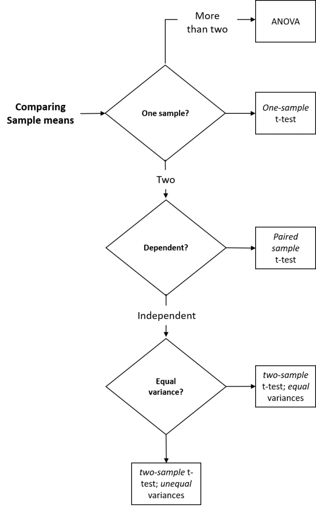
Figure 1: Summary of parametric inferential methods used to compare two sample means.
- The one-sample t-test allows us to compare the mean of a single sample with an expected mean based on prior data (or a theoretical value), to determine if they are significantly different. For example, if we – as part of an annual validation of our seed stocks – measured the mean weekly growth rate of ten seedlings from our in-house stock of spring barley seeds, we could compare this mean to last year’s mean by performing a one-sample t-test to determine whether this year’s mean growth rate was significantly different from last years recorded mean (the null hypothesis is that seedling vigor is unchanged, and that there will be no significant difference in weekly growth rate).
- The paired t-test allows us to compare two sample means if each value within one sample can be paired with an associated value in the other, to determine if they are significantly different. For example, if we measured the mean weekly growth rate of the same seedlings from our in-house stock of spring barley seeds over a period of consecutive weeks, we could compare this week’s mean to last week’s mean by performing a paired t-test to determine whether this week’s mean growth rate is significantly different from last week’s mean.
- The (unpaired) two-sample t-test allows us to compare two sample means, to determine if they are significantly different. For example, if we measured the mean weekly growth rate of herbicide-treated seedlings to untreated seedlings, we could use a two-sample t-test to determine whether the mean growth rate for the treated seedlings was significantly different from the untreated seedlings.
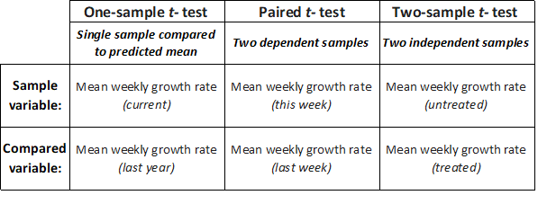
Figure 2: Example cases for one sample t-test for single data samples, paired two-sample t-test for dependent samples or two-sample t-test for independent samples.
Assumption of Normal (Gaussian) distribution
The t-test assumes that the samples follow a normal (Gaussian) distribution. A number of tests of normality are available, such as the Shapiro–Wilk and Kolmogorov–Smirnov tests, but these require statistical insight or access to statistical software packages.
A simpler graphical approximation to evaluate normality is to visually determine how closely a histogram of the sample resembles a “bell-shaped” normal probability curve (Figure 3). If the shape of the histogram looks approximately symmetrical and bell-shaped, the assumption of normalcy can be considered reasonably met. A box-plot (inset, Figure 3) also provides an overview of data distribution and can identify non-normal distributions.
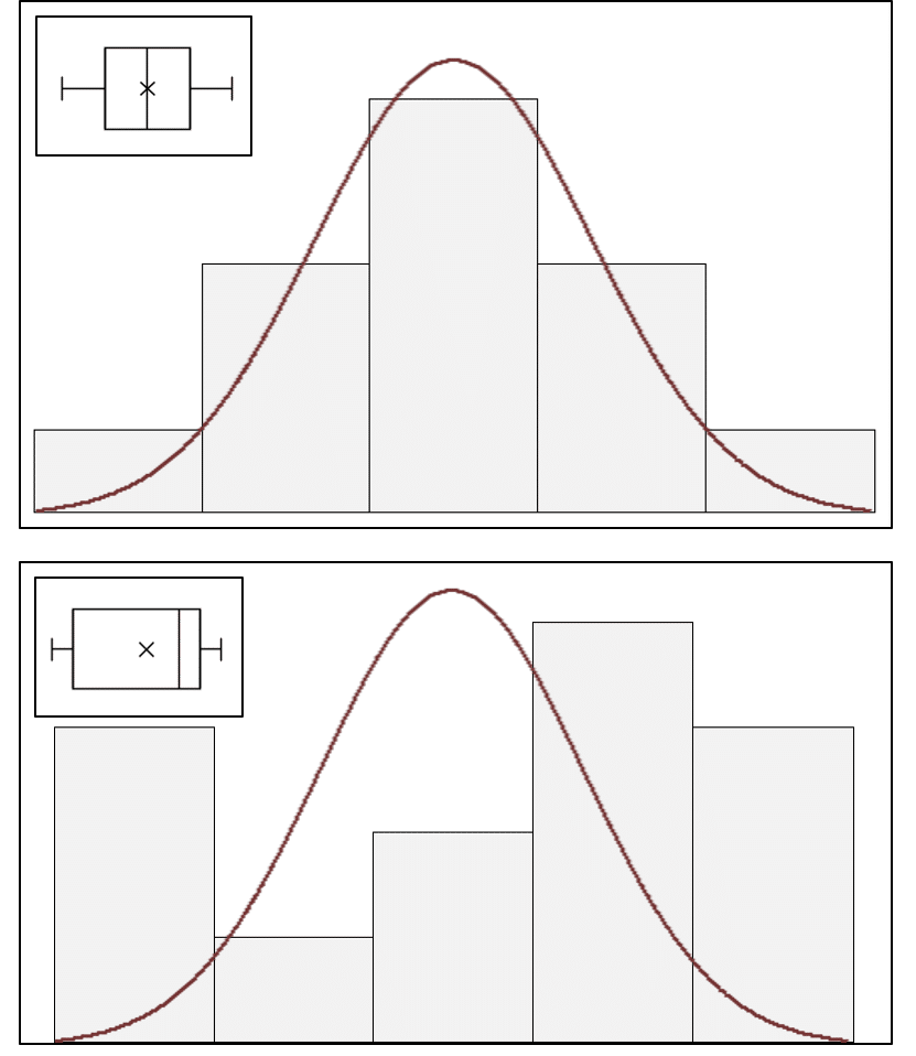
Figure 3: Histograms of sample data overlaid with a normal probability curve and box-plot (inset) identifying normal (top) and non-normal (bottom) data distributions.
A general rule of thumb is that the distribution of the mean approaches a normal distribution as sample size increases, and that to compare means your sample size should be at least 30.
For situations where a sample size of 30 is not feasible, the t-test was developed specifically to improve means testing results for small samples (typically less than 10 degrees of freedom). Especially for samples with less than 5 degrees of freedom, the sharply increasing values of t (Figure 4) compensate for small sample size tendencies toward Type I errors (claiming a difference is significant when it is not).
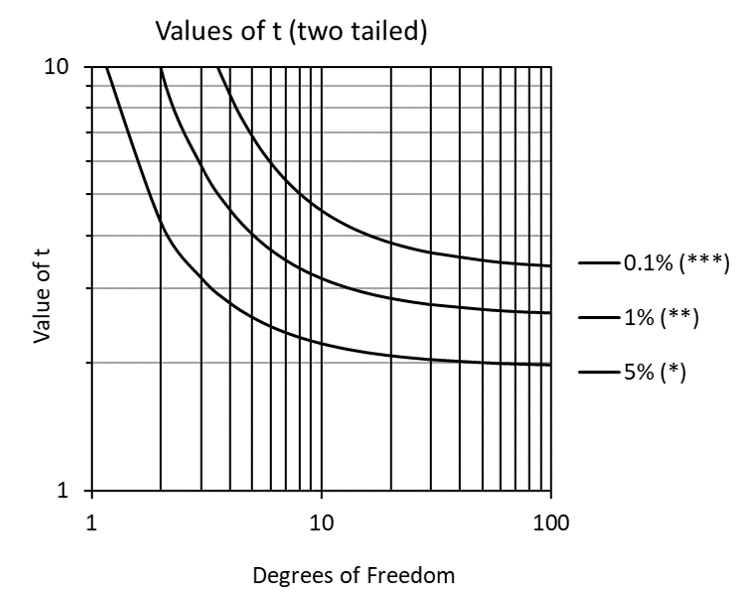
Figure 4: Values of t (two-tailed) for varying levels of significance.
If our data is not normally distributed, we have three options: to transform our data (e.g. log transformation) to normalize the distribution, to use a nonparametric test to compare the means, or simply to use the t-test despite the non-normalcy of our data (the t-test is considered to be robust to violations of assumptions of normalcy).
The (unpaired) two-sample t-test assumes that the data is sampled from populations that have equal variances, even if their means are different. As part of the (unpaired) two-sample t-test analysis, the f-test is used to determine if the two samples have equal variances – the topic of the next article. Implementation of the t-test will be discussed in article XV.
_________________________________
Thanks for reading – please feel free to read and share my other articles in this series!
The first two books in the LABCOAT GUIDE TO CROP PROTECTION series are now published and available in eBook and Print formats!
Aimed at students, professionals, and others wishing to understand basic aspects of Pesticide and Biopesticide Mode Of Action & Formulation and Strategic R&D Management, this series is an easily accessible introduction to essential principles of Crop Protection Development and Research Management.
A little about myself
I am a Plant Scientist with a background in Molecular Plant Biology and Crop Protection.
20 years ago, I worked at Copenhagen University and the University of Adelaide on plant responses to biotic and abiotic stress in crops.
At that time, biology-based crop protection strategies had not taken off commercially, so I transitioned to conventional (chemical) crop protection R&D at Cheminova, later FMC.
During this period, public opinion, as well as increasing regulatory requirements, gradually closed the door of opportunity for conventional crop protection strategies, while the biological crop protection technology I had contributed to earlier began to reach commercial viability.

