Guide to Essential Biostatistics XIX: Linear regression (PROBIT)
In the previous articles in this series, we explored the Scientific Method, Proposing Hypotheses and Type-I and Type-II errors, Designing and implementing experiments (Significance, Power, Effect, Variance, Replication, Experimental Degrees of Freedom and Randomization), Critically evaluating experimental data (Q-test; SD, SE, and 95%CI) as well as Two-Sample Means Comparisons (the t-test) and ANOVA.
Probit (“probability unit”) models were developed by American biologist and statistician Chester Bliss in 1934, as a method to evaluate dose response in pesticide data.
Probit allows researchers to convert mortality (effect) percentages to probit values, which approximate a straight line function between the logarithm of the dose and effect, and which can be analyzed by simple linear regression methods.
Probit is thus the transformation of the sigmoid dose-response curve to a straight line.
The Probit model was further adapted and tabulated at Rothamsted by British statisticians D. J. Finney and W. L. Stevens in 1948 to avoid having to work with negative probits in an era before the ready availability of electronic computing.
It is these Probit tables that even today ensure that dose-response fitting to evaluate dose-response relationships may be conveniently performed when statistical software packages are not available, and experimenters do not have a background in mathematics.
Probit analysis may be conducted using tables to determine the probits and fitting the relationship by eye or through linear regression, or by using a statistical package.
The process for evaluating dose-response relationships through the Probit analysis by hand, or by using a spreadsheet, are outlined in the following:
▶︎ Step 1: log transform the doses.
▶︎ Step 2: Convert % response to probits (short for probability unit).
Probits are generally calculated in the range where the sigmoidal response increases linearly i.e. from approximately 10-20% to 80-90% of maxima and should ideally contain three points within this linear phase.
If control (untreated) response is more than 10%, Schneider-Orelli’s correction (see previous chapter) may be used.
Probits for a given percentage effect may be determined using Finney’s table:
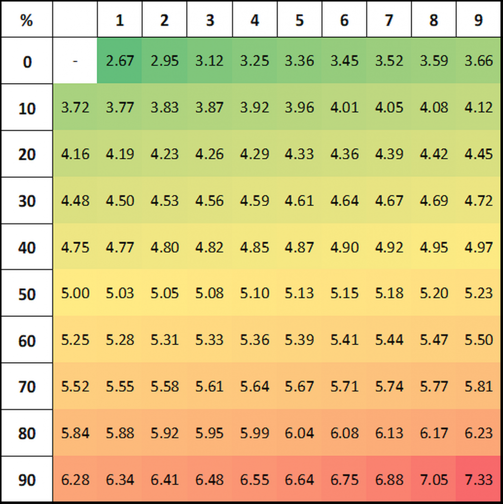
Figure 1: Finney’s table for the transformation of response percentages to probits.
In our example, for a 25% response the corresponding probit is 4.33, for 58% effect probit=5.20 and for 88% effect probit=6.18:
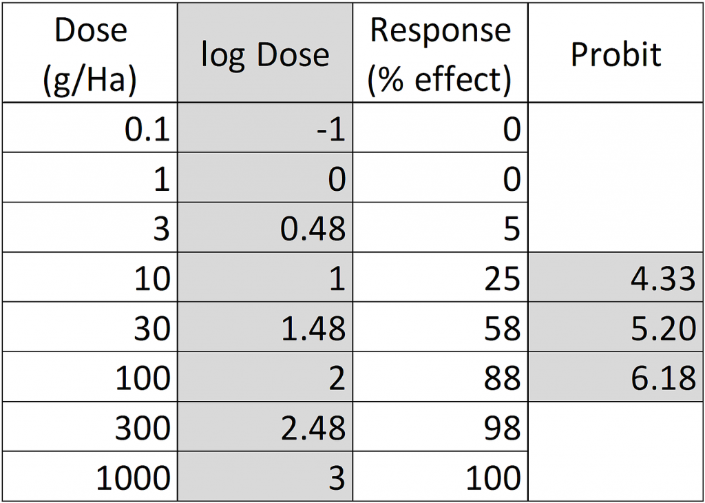
Figure 2: Dose-response data table, log-transformed doses and transformation of response percentages to probits.
▶︎ Step 3: Graph the probits versus the log of the concentrations and perform a linear regression, by hand or using a spreadsheet (Figure 3).
▶︎ Step 4: Determine the ED50.
In our example, using values from a herbicide dose-response curve, the ED50 value may be fitted by eye as logED50= 1.36 from which the dose may be determined as ED50= 10^1.36= 22.91g ai/Ha:
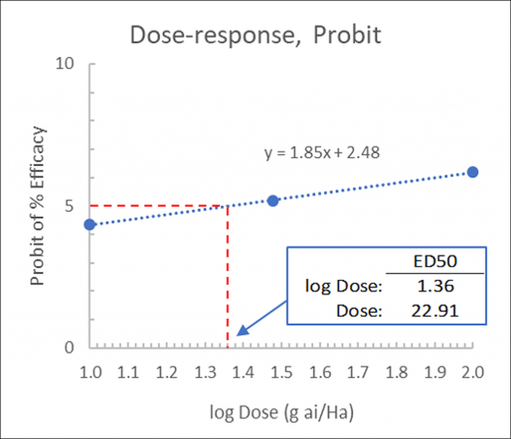
Figure 3: Linear fit of dose-response data, probits versus the log of the concentrations: visual estimation of ED50.
Alternatively, if the linear function has been calculated (in our example as y= 1.85x + 2.48) the ED50 may be calculated as:

…where 2.48 is the intercept (at x=0) and 1.85 is the slope. The Probit value is 5 for ED50 (in Finney’s table, Figure 1, for a 50% response (ED50) the corresponding probit is 5):
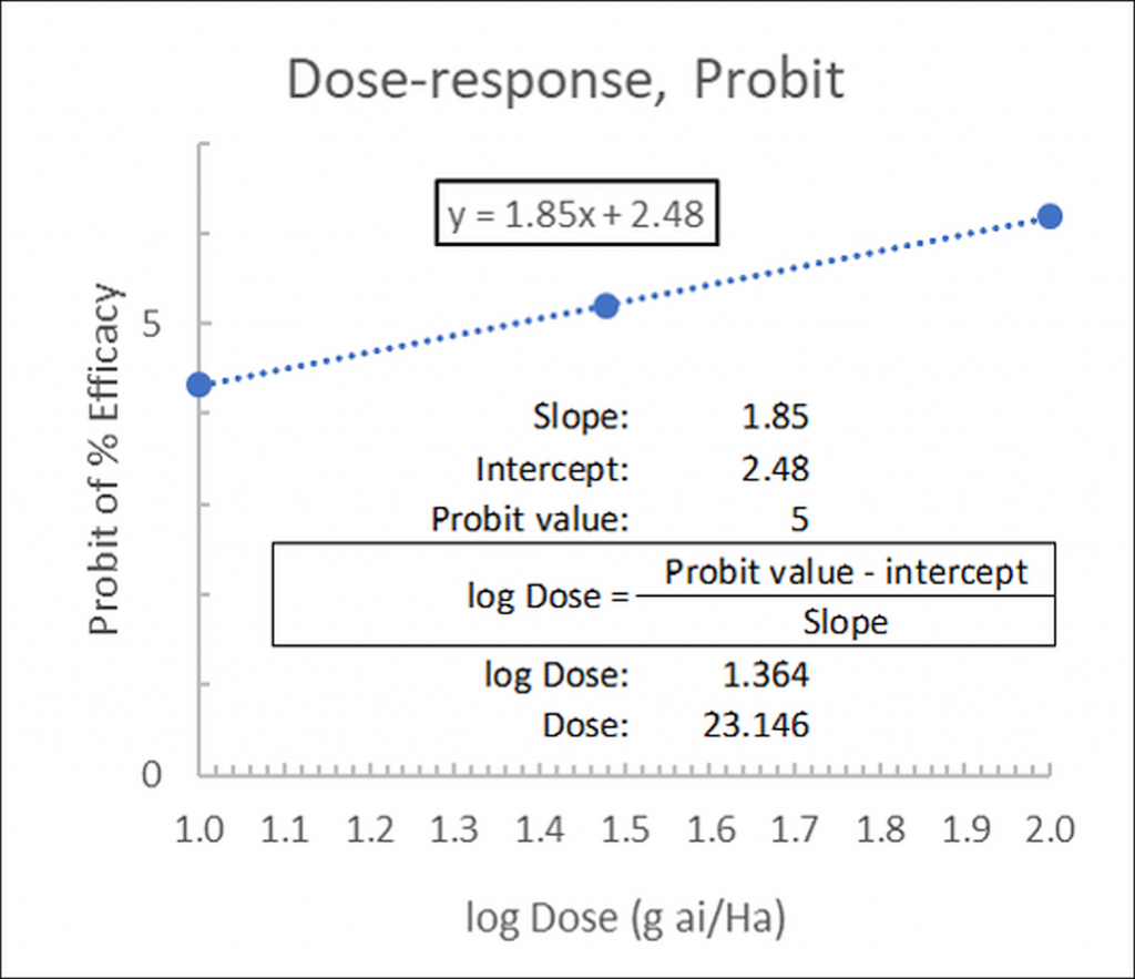
Figure 4: Linear fit of dose-response data, probits versus the log of the concentrations: calculation of ED50.
In our example, logED50= 1.364 from which the dose may be determined as ED50= 10^1.364= 23.146g ai/Ha.
An alternative method of calculating Effective Dose levels (EDx) is Logit, which can be performed through a similar process to that described for Probit.
The key difference between logit and probit models lies in the assumption of the distribution of the errors, where for probit the errors are assumed to follow a Normal distribution. In practice, both generally lead to the same conclusions and both are thus considered appropriate.
In our example, for both non-linear (sigmoidal) regression (see previous chapter) and linear (Probit) regression, both ED50 values are almost equal, and visual estimates were relatively accurate. For data with more scatter around the regression line, visual determination of ED50 becomes less precise.
As for non-linear regression, a further advantage of using statistical packages is that the goodness-of-fit of the data to the regression curve can be quantified.
Thanks for reading – please feel free to read and share my other articles in this series!
GUIDE TO ESSENTIAL BIOSTATISTICS is now published and available in eBook and Print formats!
Are you a student, researcher or science leader looking for an overview of the essential principles of Biostatistics?
Guide To Essential Biostatistics is an easily accessible primer for scientists and research workers not trained in mathematical theory, but who have previously followed a course in Biological Statistics.
This book provides a readily accessible overview on how to plan, implement and analyse experiments without access to a dedicated staff of statisticians.
Guide To Essential Biostatistics contains few calculations (the “how” of Biostatistics) but instead provides a plain-English overview of the “why” – what is it the numbers are telling us, and how can we use this to plan trials, understand our data and make decisions.
Designed to fit in a lab coat pocket for easy access, Guide To Essential Biostatistics compiles some of the most-used biostatistical techniques, approximations and rules-of-thumb used in the design and analysis of biological experiments.
Buy this book to obtain an overview of essential aspects of Biostatistics! By purchasing the print edition of this book on AMAZON, you are eligible for a FREE download of the eBook version, providing access to high-resolution, zoomable color images.
A little about myself
I am a Plant Scientist with a background in Molecular Plant Biology and Crop Protection.
20 years ago, I worked at Copenhagen University and the University of Adelaide on plant responses to biotic and abiotic stress in crops.
At that time, biology-based crop protection strategies had not taken off commercially, so I transitioned to conventional (chemical) crop protection R&D at Cheminova, later FMC.
During this period, public opinion, as well as increasing regulatory requirements, gradually closed the door of opportunity for conventional crop protection strategies, while the biological crop protection technology I had contributed to earlier began to reach commercial viability.

