Guide to Essential Biostatistics XVIII: Non-linear regression (Sigmoidal dose-responses
In the previous articles in this series, we explored the Scientific Method, Proposing Hypotheses and Type-I and Type-II errors, Designing and implementing experiments (Significance, Power, Effect, Variance, Replication, Experimental Degrees of Freedom and Randomization), Critically evaluating experimental data (Q-test; SD, SE, and 95%CI) as well as Two-Sample Means Comparisons (the t-test) and ANOVA.
Bioassays (analytical methods to determine potency of a substance by its effect on living organisms) are used in all fields of the biological sciences – from the agricultural sciences over toxicology and biochemistry to medicine – for the assessment of biological activity and selectivity of pesticides, biochemicals and pharmaceuticals.
Bioassays include dose-response studies using several (typically replicated) doses of one or more biologically active compounds, or active ingredient (a.i.) to measure the response of specific target organisms.
In dose-response experiments, an active ingredient’s (e.g. herbicide) effect on a target organism (plant) is typically investigated by constructing a dose-response curve which describes the relationship between increasing the dose and the associated change in response across a dose range.
On an arithmetic (linear) scale, the dose is plotted on the X-axis and response is plotted on the Y-axis, and the response curve is hyperbolic:
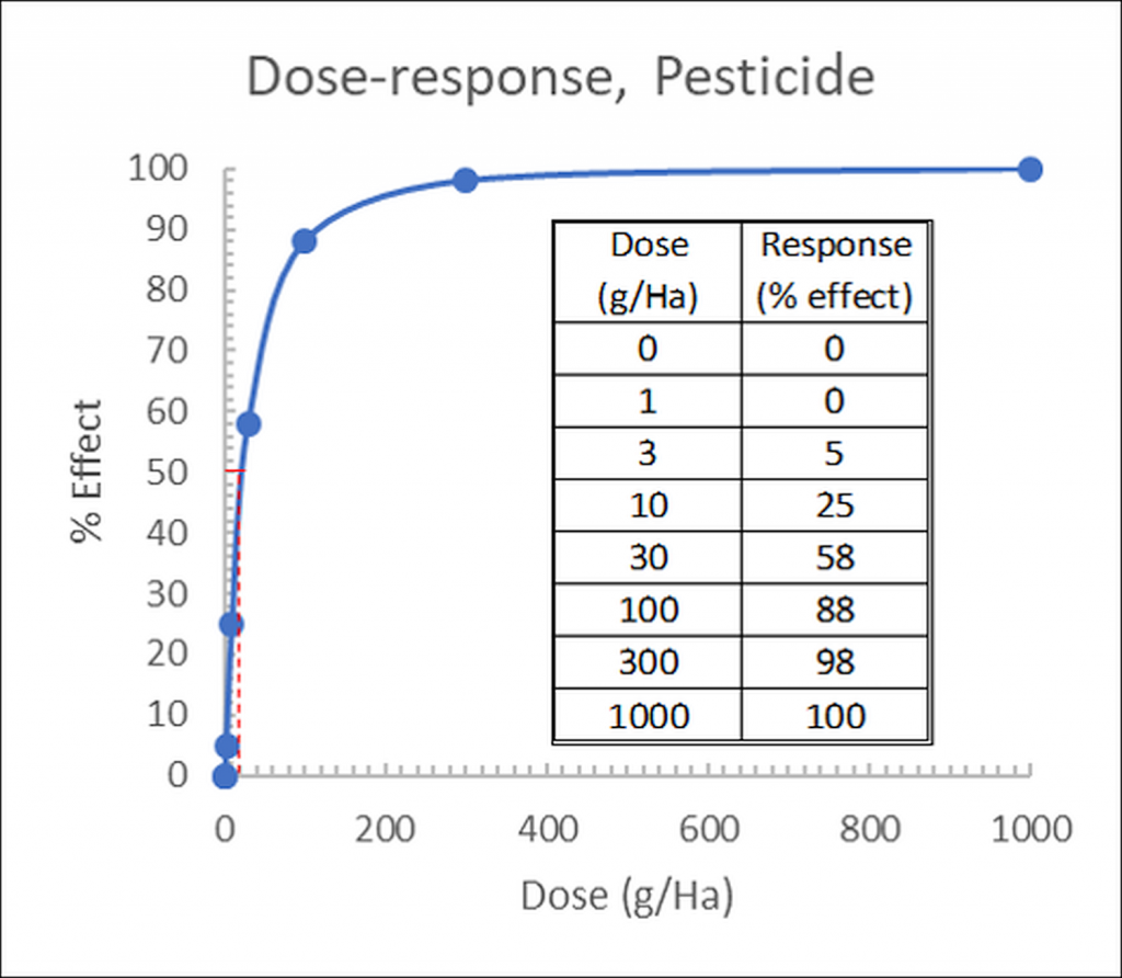
Figure 1: Hyperbolic dose-response (effect) curve for linear, arithmetic doses. Insert: Dose-response data table.
On this linear scale, it is apparent that evaluating the transition from low to high response is difficult, as most of the information is compressed in a small section of the graph.
To address this, the doses on the X-axis may be logarithmically transformed.
On a logarithmic dose scale (see Figure 18.3), dose-responses typically follow the classic sigmoidal curve familiar to biologists from e.g. bacterial growth studies.
Sigmoidal dose-response fitting
From the approximately linear slope of the sigmoidal dose-response fit (from approximately 10-20% effect to 80-90% effect, over about two log units) we can derive Effective Dose levels (EDx), i.e. the doses causing a specific response x in the target organism.
Among these are the Effective Dose, ED50 (for example, herbicide dose required to reduce for example plant growth by 50%, i.e. half-way between the upper and lower asymptote; see Figure 18.3), ED10 (dose required to reduce plant growth by 50%, often defined as the No Observable Effect Level; NOEL) and ED90.
Other terminology used includes EC (Effective Concentration), LC/LD (lethal concentration/dose, for toxicology) and IC (inhibitory concentration, for biochemistry).
Pesticide dose-response experiments typically use 5-7 doses, equally spaced on a logarithmic scale. For example, doses might be 1, 3, 10, 30, 100, 300, 1000 g ai/Ha. When converted to logarithms, these values are equally spaced: 0.0, 0.5, 1.0, 1.5, 2.0, 2.5, 3.0.
This provides a sufficiently broad and equally spaced range of doses to ensure zero percent effect at the lower asymptote (plateau) and 100% effect at the upper asymptote – requirements for fitting the sigmoidal dose-response curve (see below).
For some trials (especially insecticide trials) mortality may arise for the untreated “control” due to natural causes, and Schneider-Orelli’s formula may be used to correct for control response (typically mortality) if control response is more than 10%:
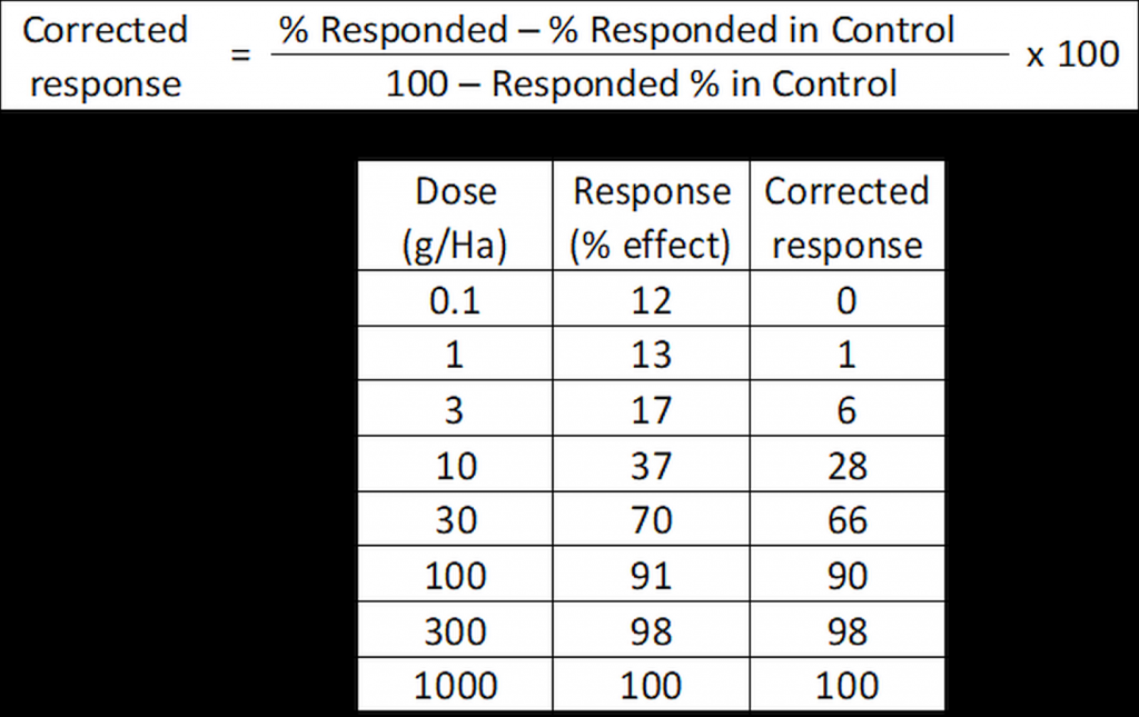
Figure 2: Schneider-Orelli’s correction for control response.
In its basic form, the standard sigmoidal dose-response curve showing response (Y) as a function of the logarithm of concentration (X) may be fitted by eye or by the following equation:

…where “Top” is the response at the upper asymptote (the response at high doses), “Bottom” is the response at the lower asymptote (response to the untreated control) and logEC50 is the logarithm of the EC50 (the dose giving a response half-way between the upper and lower asymptotes).
The number 1 indicates the standard slope (termed Hill slope) where the response increases linearly from approximately 10-20% to 80-90% of maximal as the dose increases over about two log units.
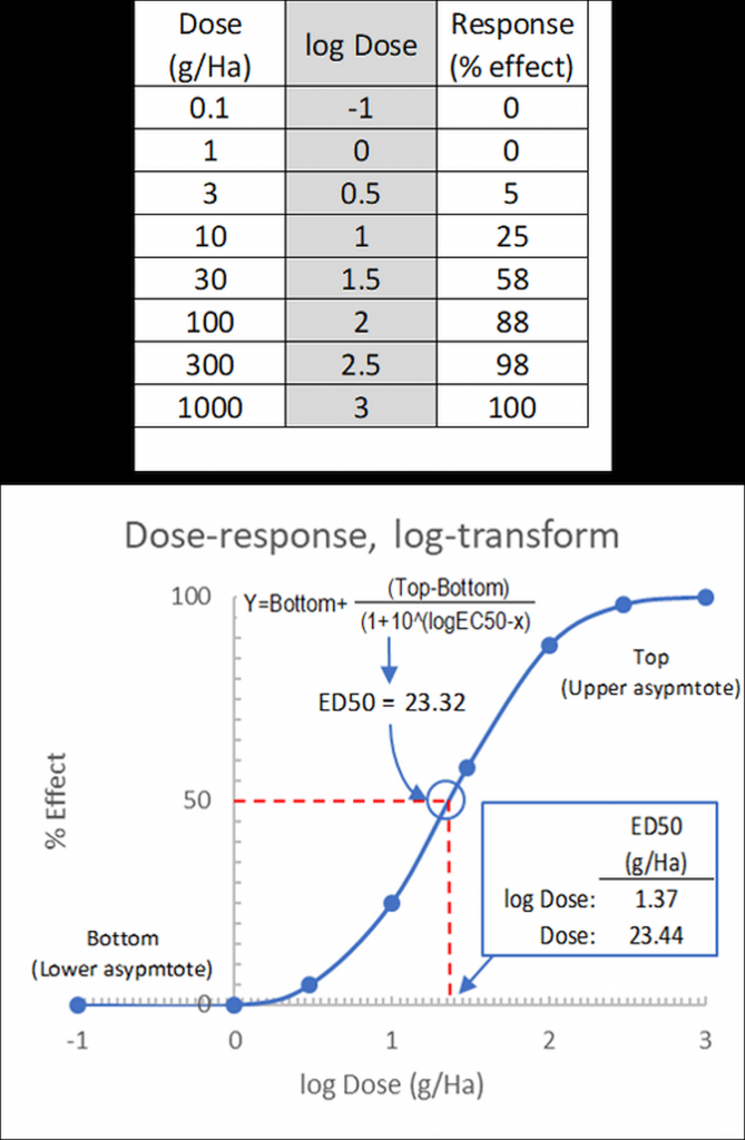
Figure 3: Sigmoidal dose-response (effect) curve for log-transformed doses, visual estimation and calculation of ED50. Top: transformed dose-response data table.
In our example above, using values from a herbicide dose-response curve, the ED50 value may be fitted by eye (Figure 18.3) as logED50 = 1.37 from which the dose may be determined as ED50 = 10^1.37 = 23.44g ai/Ha.
Alternatively, the ED50 value may be calculated (using e.g. a statistics package) as ED50 = 23.22g ai/Ha.
Here, both values are almost equal, as the data conveniently fits the sigmoidal curve – for data with more scatter around the regression line, visual determination of ED50 becomes less precise.
A further advantage of using statistical packages is that goodness-of-fit of the data to the regression curve can be quantified.
The standard sigmoidal dose-response curve assumes a standard Hill slope, but in practice, a revised equation for variable slopes is often used.
Theoretically, the slope should be equal when evaluating different formulations of the same active ingredient.
Often, however, experimenters will not have enough data to allow accurate curve fitting, and confidence intervals of the fit may be used to approach best-fit slope parameters.
These advanced cases (including biphasic dose-response curves) lie outside the scope of this book, but most statistical packages are able to fit these conditions.
If statistical software packages are not available, and experimenters do not have a background in mathematics, linear dose-response fitting may be conveniently performed using PROBIT models. This will be the topic of the next chapter.
Thanks for reading – please feel free to read and share my other articles in this series!
GUIDE TO ESSENTIAL BIOSTATISTICS is now published and available in eBook and Print formats!
Are you a student, researcher or science leader looking for an overview of the essential principles of Biostatistics?
Guide To Essential Biostatistics is an easily accessible primer for scientists and research workers not trained in mathematical theory, but who have previously followed a course in Biological Statistics.
This book provides a readily accessible overview on how to plan, implement and analyse experiments without access to a dedicated staff of statisticians.
Guide To Essential Biostatistics contains few calculations (the “how” of Biostatistics) but instead provides a plain-English overview of the “why” – what is it the numbers are telling us, and how can we use this to plan trials, understand our data and make decisions.
Designed to fit in a lab coat pocket for easy access, Guide To Essential Biostatistics compiles some of the most-used biostatistical techniques, approximations and rules-of-thumb used in the design and analysis of biological experiments.
Buy this book to obtain an overview of essential aspects of Biostatistics! By purchasing the print edition of this book on AMAZON, you are eligible for a FREE download of the eBook version, providing access to high-resolution, zoomable color images.
A little about myself
I am a Plant Scientist with a background in Molecular Plant Biology and Crop Protection.
20 years ago, I worked at Copenhagen University and the University of Adelaide on plant responses to biotic and abiotic stress in crops.
At that time, biology-based crop protection strategies had not taken off commercially, so I transitioned to conventional (chemical) crop protection R&D at Cheminova, later FMC.
During this period, public opinion, as well as increasing regulatory requirements, gradually closed the door of opportunity for conventional crop protection strategies, while the biological crop protection technology I had contributed to earlier began to reach commercial viability.

