Guide to Essential Biostatistics XVI: Inferential Statistics – ANOVA
In the previous articles in this series, we explored the Scientific Method, Proposing Hypotheses and Type-I and Type-II errors, Designing and implementing experiments (Significance, Power, Effect, Variance, Replication, Experimental Degrees of Freedom and Randomization), Critically evaluating experimental data (Q-test; SD, SE, and 95%CI) as well as Two-Sample Means Comparisons (the t-test).
While the t-test is used to compare the means of two treatments, samples or groups, Analysis of Variance (ANOVA) are hypothesis tests used to differentiate between the means of more than two treatments, or groups.
Using ANOVA to compare two groups will return the same results (p-value) as using the t-test. Although it may seem simpler to compare the means of multiple samples as a series of multiple two-sample comparisons (t-tests), this is not a recommended option as increasing the number of comparisons compounds the error, and we risk making a type-I error i.e. falsely concluding a significant difference when there is no real difference.
The objective of the ANOVA test is thus to allow us to perform a single comparison test to compare multiple groups of data, thereby reducing the chance of making a type-I error.
As the mathematics required of the ANOVA tests are beyond the scope of this article, and as the tests can now be conveniently performed through spreadsheets, online calculators and dedicated statistical programs, we will in the following focus on understanding the underlying assumptions as well as the output of the ANOVA tests.
The most common application of ANOVA in crop protection R&D is the one-way ANOVA, used to differentiate between the means of more than two treatments, for which there is one measurement variable (e.g. plant height) and one nominal variable, or factor (e.g. pesticide).
Two- and three-way ANOVA tests are used to differentiate between the means of more than two treatments, for which there is one measurement variable and two (or three) nominal variables, or factors (Figure 1).

FIGURE 1: summary of Means comparisons.
Assumption of Normality and Homogeneity of Variance
As is the case for the t–test, ANOVA assumes that the data is sampled from populations that have equal variance. Tests such as Bartlett’s test for homogeneity of variance are typically used to test this assumption – if Bartlett’s test reveals deviances from homogeneity, data transformation can be considered.
Both Bartlett’s as well as the ANOVA test assume that the samples follow a normal (Gaussian) distribution (see previous articles). A number of tests of normality are available, such as the Shapiro–Wilk and Kolmogorov–Smirnov tests, but these require statistical insight or access to statistical software packages.
If each treatment comprises less than ten data values, a general assumption (previously described as the Normality Rule of Thumb) is that any test of normal distribution will be so compromised that neither data transformation nor the use of nonparametric tests (e.g. the Kruskal-Wallis test, see previous article on “Selecting a Statistical Test) will provide a significant benefit:
▶︎ Normality Rule of Thumb: for biological data, a normal distribution may be assumed as a valid working approximation.
In daily practice, however, it is common for scientists to simply use parametric methods such as the ANOVA test directly on datasets from non-normal distributions.
Understanding the output of ANOVA tests
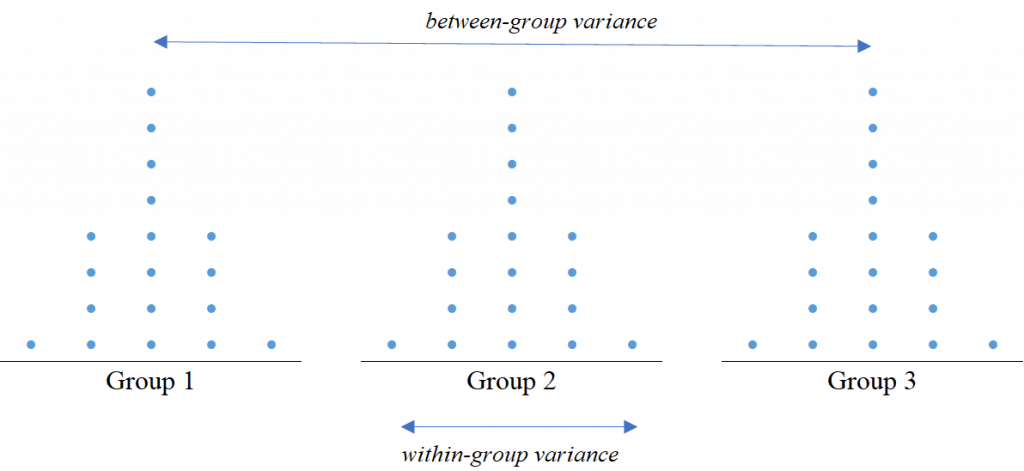
ANOVA differentiates between treatment (group) means by using the f-ratio to compare variance within and between treatments or groups – if the variation (typically termed “error”) within groups is greater than the variation between groups, the difference between the means is not considered significant.

FIGURE 2: between-group and within-group variance.
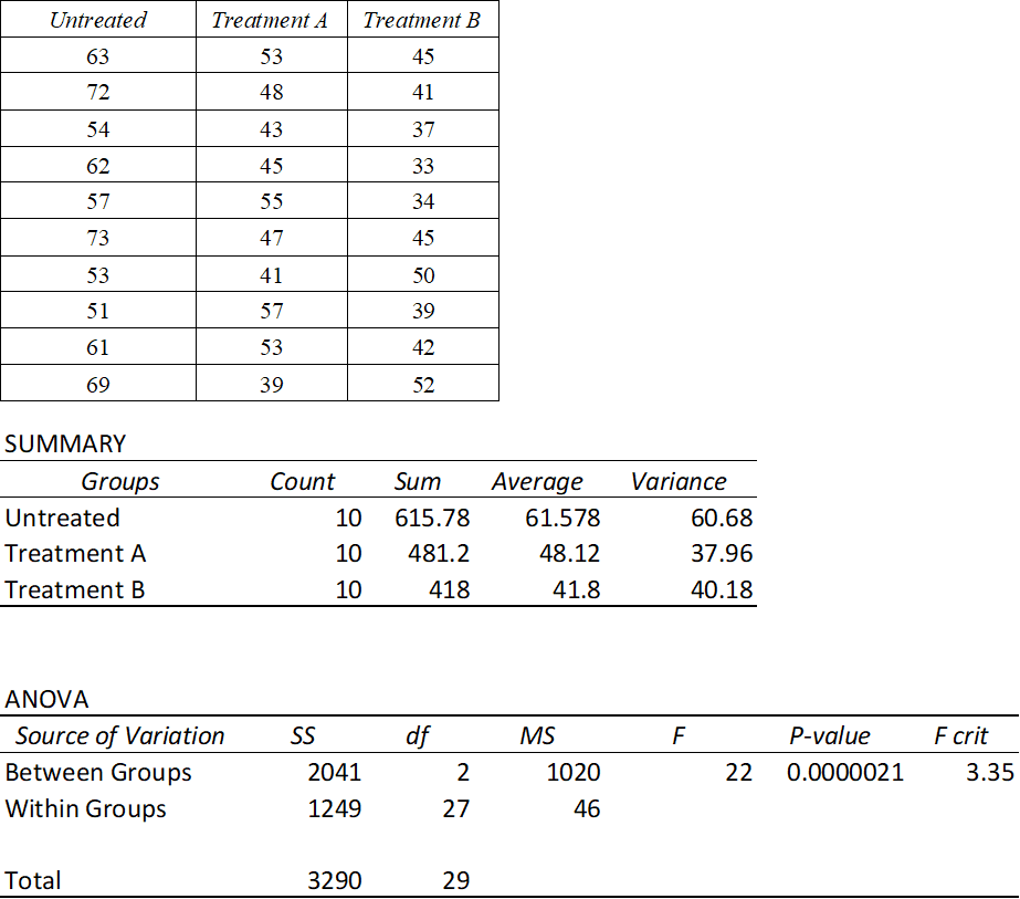
In the following example, we use the dataset for plant heights for ten untreated seedlings and ten herbicidally-treated seedlings (Treatment A) used in the previous chapter and expand it by adding an extra treatment (Treatment B), for a total of three groups (untreated control plus two treatments).

FIGURE 3: ANOVA output (Excel) comparing plant heights (cm) of untreated and treated plants.
To calculate the within-group and between-group variance, the dispersion of the data (Sum of Squares; SS) was divided by the Degrees of Freedom (df) to give the variance (Mean Square; MS).
Degrees of freedom are calculated between groups (m-1) as 3 groups minus 1 = 2 and within groups (n-m ) as 30 observations (n) minus 3 groups (m) = 27.
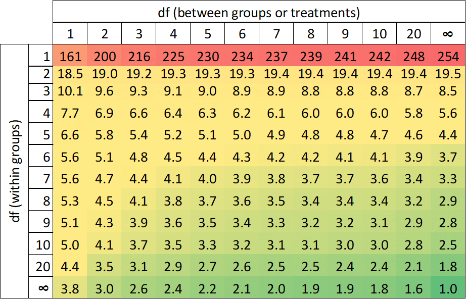
The f-ratio (F) is the ratio of the between-groups variance (MS_between) divided by the within-groups variance (MS_within), and the calculated ratio is compared to distribution values (one-tail critical f-table values) in order to determine significance (Figure 4).
As the f-ratio of the between-groups variance relative to the within-groups variance (F = 22) is greater than the table value of 3.35 for 2 df between groups and 27 df within groups, we may conclude that there is a significant difference between the means of the treatments being compared.
For manual calculations of the f-ratio, significance may be determined using the f-table:

Figure 4: One-tailed f-table for α = 0.05
However, statistical packages, spreadsheets and online ANOVA calculators supplement f-ratios and critical values with a P value (the chance that the means are equal).
If the p-value is less than 0.05, we may reject the null hypothesis that the means are equal and conclude that there is a significant difference between the means.
Likewise, if the p-value is greater than 0.05, we may accept the null hypothesis and conclude that there is no significant difference between the means.
In our example above, we can determine that the p-value is considerably less than 0.001 (i.e. the difference between the means is extremely significant). However, the results of the ANOVA test only indicate if there is a significant difference between means, and do not reveal which group is different nor how it is different.
To determine this, we need to supplement the ANOVA test with post-hoc (“done after the event”) or post-ANOVA tests for significant differences – the subject of the next article.
_________________________________
Thanks for reading – please feel free to read and share my other articles in this series!
The first two books in the LABCOAT GUIDE TO CROP PROTECTION series are now published and available in eBook and Print formats!
Aimed at students, professionals, and others wishing to understand basic aspects of Pesticide and Biopesticide Mode Of Action & Formulation and Strategic R&D Management, this series is an easily accessible introduction to essential principles of Crop Protection Development and Research Management.
A little about myself
I am a Plant Scientist with a background in Molecular Plant Biology and Crop Protection.
20 years ago, I worked at Copenhagen University and the University of Adelaide on plant responses to biotic and abiotic stress in crops.
At that time, biology-based crop protection strategies had not taken off commercially, so I transitioned to conventional (chemical) crop protection R&D at Cheminova, later FMC.
During this period, public opinion, as well as increasing regulatory requirements, gradually closed the door of opportunity for conventional crop protection strategies, while the biological crop protection technology I had contributed to earlier began to reach commercial viability.


