Guide to Essential BioStatistics X: Critically evaluating experimental data – Descriptive Statistics: SD, SE or 95%CI?
In this tenth article in the LabCoat Guide to BioStatistics series, we learn about Descriptive Statistics: SD, SE and 95%CI.
In the previous articles in this series, we explored the Scientific Method and Proposing Hypotheses and Type-I and Type-II errors, Designing and implementing experiments (Significance, Power, Effect,Variance, Replication, Experimental Degrees of Freedom and Randomization).
In the following articles we will explore: Critically evaluating experimental data (Q-test; SD, SE and 95%CI), and Concluding whether to accept or reject the hypothesis (F- and T-tests, Chi-square, ANOVA and post-ANOVA testing).
Once we have identified possible outliers (due to biological variance or experimental malfunction) and eliminated them as appropriate (see previous article), we are ready to continue the critical evaluation of our experimental data in the form of Descriptive Statistics.
Descriptive Statistics are used to describe the basic features of our experimental data and, together with graphical representations, can provide simple summaries about the Variability, Means, and Significance of our data.
The most common descriptive statistics used in the biological sciences are those of sample Standard Deviation (SD), Standard Error of the Mean (SEM) and 95% Confidence Intervals (95%CI).
Sample Standard Deviation (SD) is used to quantify variability in the experimental data and is expressed in the same units as the data. While calculators and spreadsheets can calculate Standard Deviation at the click of a button, it is occasionally useful to be able to give a rough estimate of the Standard Deviation of a data set using the Range Rule of Thumb:
▶︎ Range Rule of Thumb: SD ≈ Range/4 where Range = (maximum value) – (minimum value).
This rule of thumb provides a useful estimation for samples sizes greater than n=12. For many biological trials, sample sizes are smaller, and division by 3 (for n = 8-12) or 2 (for n < 7) provides a better estimate (see earlier article).
The Standard Deviation cannot be used to determine whether the difference between Means is significant and can only be used to express variability or to derive the Standard Error of the Mean or its extension, the 95% Confidence Interval.
An example of a practical application of quantifying variability in a trial is given in figure 10.1, where it is apparent that the variability is different for each data point.
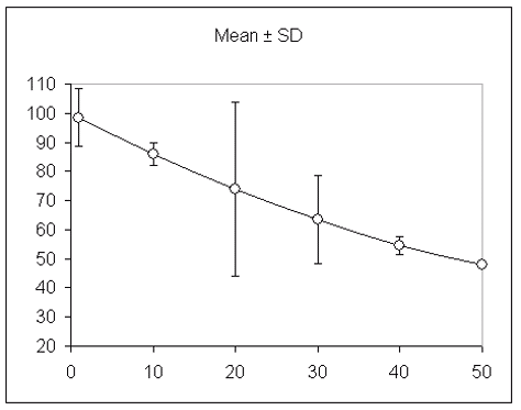
Figure 10.1: differences in variability within a trial, expressed as Mean ± SD
Accordingly, we can deduce that some independent factor (variance within the biological material being tested, researcher variance, equipment variance or climatic variance) contributed to variability and that we should return to our experimental setup to identify and remove this disturbance.
From personal experience I can confirm that if you do not address this yourself, a reviewer will almost certainly insist that this experiment is repeated, leading to a significant delay in publication of e.g. a scientific article.
Standard Error of the Mean (SE or SEM) is derived from the Standard Deviation and quantifies the precision of the calculated Mean relative to the true population Mean, and considers the variability (Standard Deviation, SD) and the sample size (n) – factors which determine how close the sample Mean will be relative to the population Mean.
As for Standard Deviation, Standard Error of the Mean is expressed in the same units as the data, and is calculated as the Standard Deviation divided by the square root of the sample size:
SE = SD / SQRT(n)
It can be seen from the above equation that the Standard Error is always smaller than the Standard Deviation of a dataset and, in contrast to the Standard Deviation, the Standard Error always gets smaller as your sample size gets larger.
For this reason, Standard Error of the Mean is sometimes misused for data description, and it is generally recommended that 95% Confidence Intervals be used instead.
The 95% Confidence Interval (95%CI) is derived from the Standard Error of the Mean and quantifies the precision of the calculated Mean, such that the Confidence Interval contains the true population Mean with 95% certainty.
The 95% Confidence Interval of a Mean is calculated as the Standard Error of the Mean multiplied by a constant from the t-distribution for the given sample size (n degrees of freedom, DF):
95%CI = SEM * t(n)

Figure 10.2: t-distributions for given sample sizes (n degrees of freedom, DF) for the calculation of 95% Confidence Intervals.
While 95% Confidence Intervals are easily calculated, it is occasionally useful to be able to give a rough estimate of these Intervals using the Confidence Interval Rule of Thumb:
▶︎ Confidence Interval Rule of Thumb I: for large sample sizes, 95% Confidence Interval may be estimated from the Mean plus or minus two Standard Errors of the Mean.
The above is valid for large sample sizes, for smaller sample sizes the t-distribution provides a correction factor. Referring to the t-distribution (Figure 10.2) we can see that t-values are close to two for datasets greater than twenty while for datasets less than 10 the t-value increases rapidly.
Plotting and interpreting SD, SEM and 95%CI Error bars
When plotting data with Error bars or creating tables with +/- values, SD, SEM, and 95%CI are often applied and interpreted incorrectly. Almost as frequently, Error bars are presented without any mention of what they indicate.
Let us begin by calculating the Mean Standard Deviation, Standard Error of the Mean and 95% Confidence Interval of a set of data. In the following example, the Mean is illustrated by use of a bar graph, to which the respective Error bars are added.
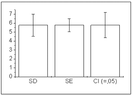
Figure 10.3: bar graph for the Mean of a dataset showing Error bars for Standard Deviation (SD), Standard Error of the Mean (SE) and 95% Confidence Interval (CI), respectively.
As we can see, the Standard Deviation Error bars are broader (further from the Mean) than those of the Standard Error of the Mean. This is because the Standard Error of the Mean is calculated as the Standard Deviation divided by the square root of the sample size.
For this reason, Standard Errors of the Mean are sometimes presented as Error bars without any indication of their identity, with the intent of making variability seem as small as possible. Even worse, this practice may mislead those who erroneously interpret non-overlapping Error bars as indicative of significant differences between the Means.
Standard Deviations should only ever be used to express the variation in our data and showing the variation in our data as a scatter plot usually provides more information then expressing the variation as Standard Deviation Error bars. SEM Error bars may be used to express how accurately your data define the Mean, but if your objective is to compare Means, 95% Confidence Interval Error bars are more useful.
In addition, Confidence Intervals may be used to provide an initial estimate of statistical significance, and Confidence Intervals are often easier to interpret than statements about statistical significance. As an initial indication, if Confidence Intervals do NOT overlap, the Means are probably significantly different (at the P<0.05 level). This may be confirmed as required using a valid statistical test (e.g., a two-sample t-test).
It is important to be aware that the opposite is not necessarily true (a mistake made by students and scientists alike): if Confidence Intervals DO overlap, there may be a statistically significant difference between the Means, and it is thus NOT possible to deduce that the difference between the Means are NOT significant.
However, a statistical rule of thumb states that if Confidence Interval Error bars overlap by more than 25%, the Means are probably not significantly different at the p < .05 level) – to confirm this one should conduct a two-sample t-test and calculate the p-value.
▶︎ Confidence Interval Rule of Thumb II: if Confidence Interval Error bars do not overlap, the differences between the Means are probably significant; if Confidence Interval Error bars overlap by more than 25%, the differences between the Means are probably not significant.
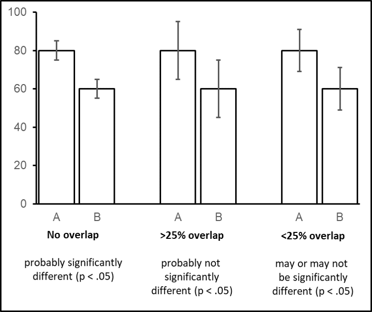
Figure 10.4: use of 95% Confidence Interval (95%CI) Error bars to estimate the significance of differences between Means.
In conclusion: when used correctly, Standard Deviation, Standard Error of the Mean and 95% Confidence Intervals are useful descriptive statistics allowing us to critically evaluate our experimental data for variability (SD), proximity of the calculated Mean to the population Mean (SE) and may be used as a visual estimate of whether the differences between Means are significant (95%CI).
The principal advantage (and potential disadvantage) of using 95% Confidence Intervals to estimate the significance of differences between Means is that these calculations may be easily performed and interpreted without access to – or an understanding of – advanced statistical techniques.
Thanks for reading – please feel free to read and share my other articles in this series!
The first two books in the LABCOAT GUIDE TO CROP PROTECTION series are now published and available in eBook and Print formats!
Aimed at students, professionals, and others wishing to understand basic aspects of Pesticide and Biopesticide Mode Of Action & Formulation and Strategic R&D Management, this series is an easily accessible introduction to essential principles of Crop Protection Development and Research Management.
A little about myself
I am a Plant Scientist with a background in Molecular Plant Biology and Crop Protection.
20 years ago, I worked at Copenhagen University and the University of Adelaide on plant responses to biotic and abiotic stress in crops.
At that time, biology-based crop protection strategies had not taken off commercially, so I transitioned to conventional (chemical) crop protection R&D at Cheminova, later FMC.
During this period, public opinion, as well as increasing regulatory requirements, gradually closed the door of opportunity for conventional crop protection strategies, while the biological crop protection technology I had contributed to earlier began to reach commercial viability.

