Guide to Essential BioStatistics IX: Critically evaluating experimental data – the Q-test for the identification of outliers
In this ninth article in the LabCoat Guide to BioStatistics series, we learn about the Q-test for the identification of outliers.
In the previous articles in this series, we explored the Scientific Method and Proposing Hypotheses and Type-I and Type-II errors, Designing and implementing experiments (Significance, Power, Effect,Variance, Replication, Experimental Degrees of Freedom and Randomization).
In the following articles we will explore: Critically evaluating experimental data (Q-test; SD, SE and 95%CI), and Concluding whether to accept or reject the hypothesis (F- and T-tests, Chi-square, ANOVA and post-ANOVA testing).
In one of the first articles in this series, we began with the observation that a herbicide safener might reduce insecticide phytotoxicity, from which a research hypothesis was formulated.
To experimentally test the hypothesis we used significance levels, power, and effect to design a randomized complete block experiment in which plants were treated with insecticides in the absence or presence of safeners and evaluated for differences in phytotoxicity between treatments.
The experimental parameters were defined under the assumption that our data would be derived from an approximately normal data set. We learned that for biological data, the assumption of normality is generally a valid approximation, as the normal distribution of biological data is surprisingly ubiquitous.
With the results of our evaluation in hand, the next step is to critically evaluate the experimental data by identifying and possibly rejecting outliers. Before proceeding, we should ensure that all values are correctly entered, and correct if necessary.
The next step is to take experimental problems into account – if an apparent outlier derives from an experimental mistake or malfunction, it may be justified to exclude the value without performing additional calculations.
It should be noted that in addition to detecting outliers with the intention of eliminating them from subsequent statistical analyses, there is also the option of detecting outliers to identify datasets that qualify for retesting, or to identify outliers with the intention of retaining them for analysis using so-called robust statistical techniques.
The need to identify and remove outliers is reduced when the data is to be analyzed using “robust” methods of statistical analysis, such as nonparametric tests which compare the distribution of ranks.
Here the largest value will have the highest rank irrespective of how large that value is. If the data is to be statistically analyzed using parametric tests (which assume a Gaussian distribution, or Normalcy) the need to eliminate outliers is far greater.
The simplest method to identifying outliers in smaller datasets (n = 3-10) typical for biological trials is to use the Q-test developed by Dean and Dixon, for which we again assume Normalcy of our data (the Q-test prescribes that the data – excluding the possible outlier – must be Normally distributed).
We begin by arranging the data in order of increasing value and calculate Q as the Gap divided by the Range, where the Gap is the difference between the outlier and the closest number to it and the Range is the difference between the lowest and the highest value.
Q = GAP / RANGE
The null hypothesis for the Q-test is: there are no outliers in the dataset. If the value of Q is higher than the associated table value corresponding to the sample size and Confidence level (typically the 95% Confidence level, alpha = 0.05), the outlier may be rejected.
In the following experimental dataset, we wish to determine whether the value 77 is an outlier at the 95% Confidence level.
After sorting the data into ascending order, we can use the following formula to calculate the Q statistic by dividing the gap (5) by the range (10)
Q = GAP / RANGE = 5 / 10 = 0.5
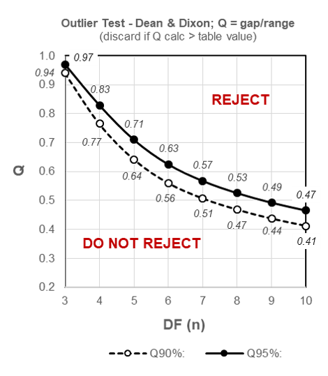
From the schematized table of critical values for Q (below) we can quickly determine that our calculated Q statistic of 0.5 is less than the critical two-sided (i.e. determining for outliers at both extremes of the dataset) table value of 0.53 for a sample size of 8 at the most commonly used 95% Confidence level, and the data value 77 may thus NOT be rejected:
Figure 9.1: Outliers – schematized two-sided table for critical values of Q for 90% and 95% Confidence levels.
The Q-test for outliers is a mathematically simple procedure but does require that we take the time to consider the results logically: for example, performing the Q-test on the values 82.24; 82.25 and 82.25 returns the conclusion that 82.24 is an outlier! Clearly, statistical significance does not always equal practical significance.
An alternative method in common use for larger datasets is Grubb’s test for outliers, in which outliers are identified as the difference between the outlier and the Mean, divided by the Standard Deviation.
This ratio is then compared to a table of critical values. The advantage of the Q-test relative to Grubb’s test is that calculations may easily be made by hand, the disadvantage is that it is only valid for data sets up to n=10. However, for most experimental biological applications the Q-test is both appropriate and convenient.
Thanks for reading – please feel free to read and share my other articles in this series!
The first two books in the LABCOAT GUIDE TO CROP PROTECTION series are now published and available in eBook and Print formats!
Aimed at students, professionals, and others wishing to understand basic aspects of Pesticide and Biopesticide Mode Of Action & Formulation and Strategic R&D Management, this series is an easily accessible introduction to essential principles of Crop Protection Development and Research Management.
A little about myself
I am a Plant Scientist with a background in Molecular Plant Biology and Crop Protection.
20 years ago, I worked at Copenhagen University and the University of Adelaide on plant responses to biotic and abiotic stress in crops.
At that time, biology-based crop protection strategies had not taken off commercially, so I transitioned to conventional (chemical) crop protection R&D at Cheminova, later FMC.
During this period, public opinion, as well as increasing regulatory requirements, gradually closed the door of opportunity for conventional crop protection strategies, while the biological crop protection technology I had contributed to earlier began to reach commercial viability.


